Jonathan Dobres

I’ve been thinking more about data visualization, if the previous post wasn’t enough of an indication. I recently stumbled upon an interesting post by Sean Lorenz at the Domino Data Lab blog on how to use R’s ggmap package to put stylish map tiles into your visualizations.

In the midst of his engaging and accessible tour of the package, Lorenz offers the following visualization of fatal motor vehicle collisons by state (or at any rate, a version very similar to the one I have here). Click to embiggen:

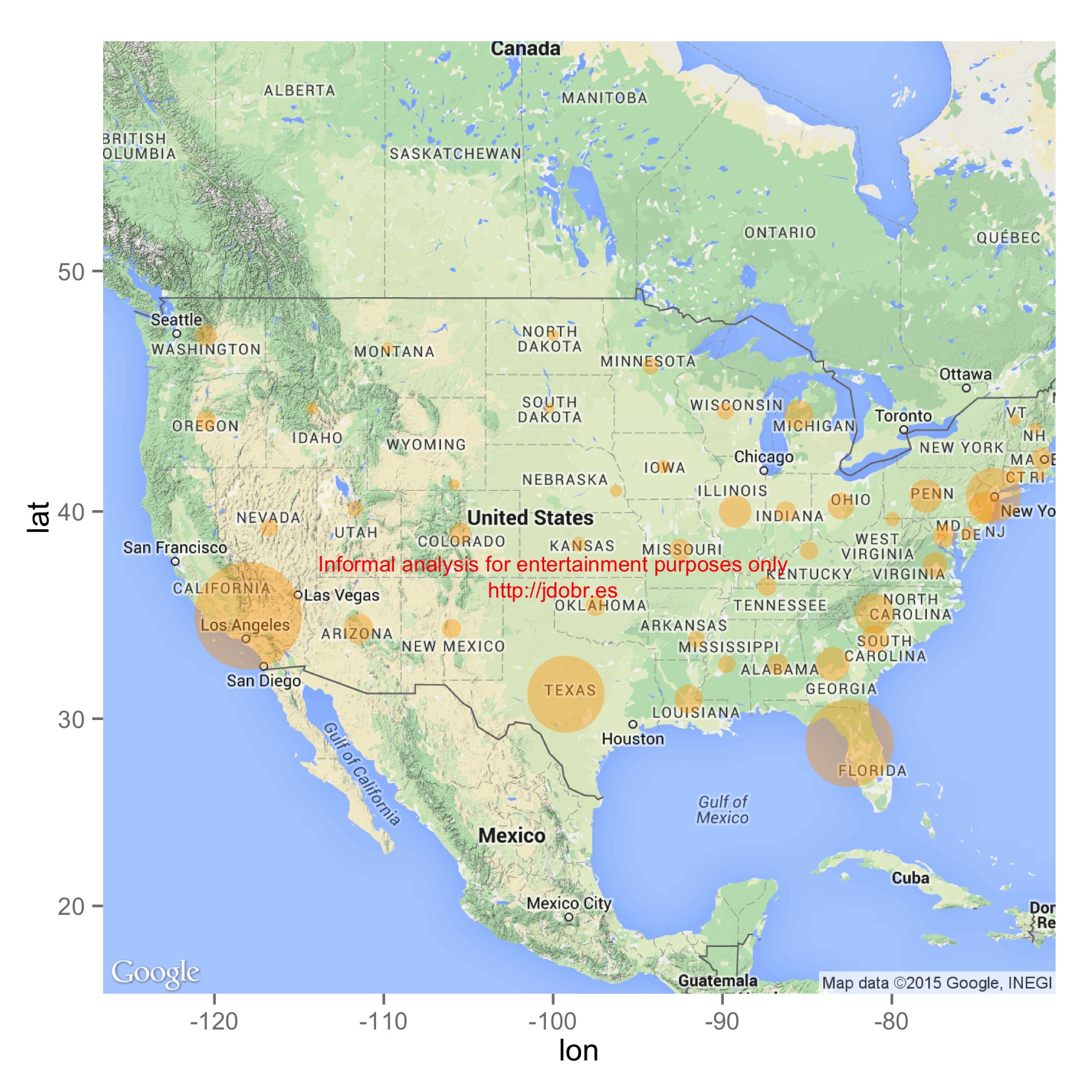
Lorenz says that this is a nice visualization of “the biggest offenders: California, Florida, Texas and New York.” But something about that list of states in that particular order seemed somehow familiar, and caught my attention.

Disclaimer

Before I continue, I’d like to state that the following is an informal analysis. It is intended for entertainment and educational purposes only, and is not scientifically rigorous, exhaustive, or in any way conclusive.

Data and R code for this project are available in my Github repository.

What Were We Talking About?

So, back to that map. The one where California, Florida, Texas, and New York were the “biggest offenders”. This struck me as suspicious, as California, Florida, Texas, and New York are coincidentally the most populous states in the country (in that order). A close reading of Lorenz’s post shows that he is, indeed, working with the raw number of collisions per state, and is not normalizing by the states’ populations. That’s important because, as you can see, there’s a very strong relationship between the number of people in a state and the number of accidents:

With a relationship that strong (even removing the Big Four outliers, R² = 0.80), a plot of raw motor vehicle accidents is essentially just a map of population. Dividing the number of collisions per state by that state’s population yields a very different map:

As you can see, many of the bubbles are now roughly the same size. Florida still stands out from the crowd, and there’s a state somewhere in the Northeast with a very high accident rate, though it’s hard to tell which one, exactly. This map is no longer useful as a visualization, because it’s no longer clarifying the relationships between the data points. This is the main problem with bubble maps: they often visualize data that do not actually have a meaningful spatial relationship, and they do so in a way that would be hard to examine even without the superfluous geography.

So how else might we visualize this information? Well, how about a chloropleth map, with each state simply colored by accident rate:

The brighter the state, the higher the rate.¹ Here, it’s more obvious that Delaware, New Mexico, Louisiana, and Florida have high accident rates, but which has the highest? And what about that vast undifferentiated middle? Maybe the problem is that all those subtle shades of blue are hard to tell apart. Maybe we should simplify the coloring and bin the data into quantiles?

Colorful, and simpler, but not necessarily more useful. From this map, you’d get the impression that Florida, Delaware, Texas, California, and many other states all have comparable accident rates, which isn’t necessarily true. How about we ditch our commitment to maps and just plot the data points?

Ah, clarity at last. Here I’m still coloring the points by quantile so that you can see how much of the data’s variability was hidden in the previous map. Now it’s immediately clear that Delaware, New Mexico, Florida, Louisiana, and South Carolina all have unusually high accident rates (arguably, so do North Carolina and Arizona). Beyond that, almost every other state clusters within one standard deviation of the national average, with South Dakota having a notably low accident rate.

Of course, Lorenz’s point wasn’t really about the accident data, it was about how nifty maps can be. Having just spent the last few paragraphs demonstrating the ways in which maps can fool us, you might get the impression that I’m down on maps. I’m really not. Maps can be beautiful and informative, but by definition, they need to show us data with some spatial relevance. Take, for instance, this map of the Boston marathon.

The lovely tiles are pulled from Stamen Maps, courtesy of the ggmap package, and I really can’t emphasize enough how much work ggmap is doing for you here.² From there, it was pretty easy to overlay some custom data. The red line traces the path of the Boston Marathon, and the blue line shows Boston’s city limits. Curiously, very little of the Boston Marathon actually happens in Boston. Starting way out west in Hopkinton, the marathon doesn’t touch Boston proper until it briefly treads through parts of Brighton. Then the route passes through Brookline (a separate township from Boston, and quite ardent about it), before re-entering the city limits near Boston’s Fenway neighborhood, just a couple of miles from the finish line.